The Protein Data Bank (PDB) is the main repository of biomolecular structure data. We can use the PDB archive to understand the shape of biomolecules and understand how they work. Let’s see what’s in it:
Rows: 6 Columns: 9
── Column specification ────────────────────────────────────────────────────────
Delimiter: ","
chr (1): Molecular Type
dbl (4): Integrative, Multiple methods, Neutron, Other
num (4): X-ray, EM, NMR, Total

ℹ Use `spec()` to retrieve the full column specification for this data.
ℹ Specify the column types or set `show_col_types = FALSE` to quiet this message.
protein =data.frame(protein_file, row.names=1)protein
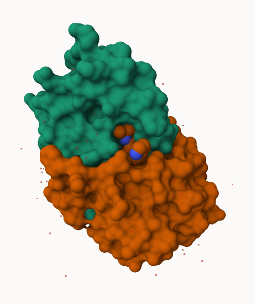
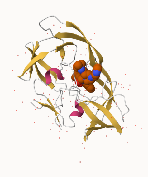
Q. Generate and insert an image of the HIV-Pr cartoon colored by secondary structure, showing the inhibitor (ligand) in spacefill.
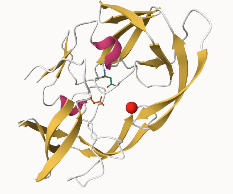
Q. One final image showing catalytic APS 25 as ball and stick and the all-important active site water molecule as spacefill
The Bio3D package for structural bioinformatics
library(bio3d)
hiv <-read.pdb("1hsg")
Note: Accessing on-line PDB file
hiv
 Call:  read.pdb(file = "1hsg")

   Total Models#: 1
     Total Atoms#: 1686,  XYZs#: 5058  Chains#: 2  (values: A B)

     Protein Atoms#: 1514  (residues/Calpha atoms#: 198)
     Nucleic acid Atoms#: 0  (residues/phosphate atoms#: 0)

     Non-protein/nucleic Atoms#: 172  (residues: 128)
     Non-protein/nucleic resid values: [ HOH (127), MK1 (1) ]

   Protein sequence:
      PQITLWQRPLVTIKIGGQLKEALLDTGADDTVLEEMSLPGRWKPKMIGGIGGFIKVRQYD
      QILIEICGHKAIGTVLVGPTPVNIIGRNLLTQIGCTLNFPQITLWQRPLVTIKIGGQLKE
      ALLDTGADDTVLEEMSLPGRWKPKMIGGIGGFIKVRQYDQILIEICGHKAIGTVLVGPTP
      VNIIGRNLLTQIGCTLNF

+ attr: atom, xyz, seqres, helix, sheet,
        calpha, remark, call
head(hiv$atom)
  type eleno elety  alt resid chain resno insert      x      y     z o     b
1 ATOM     1     N <NA>   PRO     A     1   <NA> 29.361 39.686 5.862 1 38.10
2 ATOM     2    CA <NA>   PRO     A     1   <NA> 30.307 38.663 5.319 1 40.62
3 ATOM     3     C <NA>   PRO     A     1   <NA> 29.760 38.071 4.022 1 42.64
4 ATOM     4     O <NA>   PRO     A     1   <NA> 28.600 38.302 3.676 1 43.40
5 ATOM     5    CB <NA>   PRO     A     1   <NA> 30.508 37.541 6.342 1 37.87
6 ATOM     6    CG <NA>   PRO     A     1   <NA> 29.296 37.591 7.162 1 38.40
  segid elesy charge
1  <NA>     N   <NA>
2  <NA>     C   <NA>
3  <NA>     C   <NA>
4  <NA>     O   <NA>
5  <NA>     C   <NA>
6  <NA>     C   <NA>
We need one package from BioConductor. To set this up we need to first install a package called “BiocManager” from CRAN.
Now we can use the install() function from this package like this: BiocManager::install("msa")
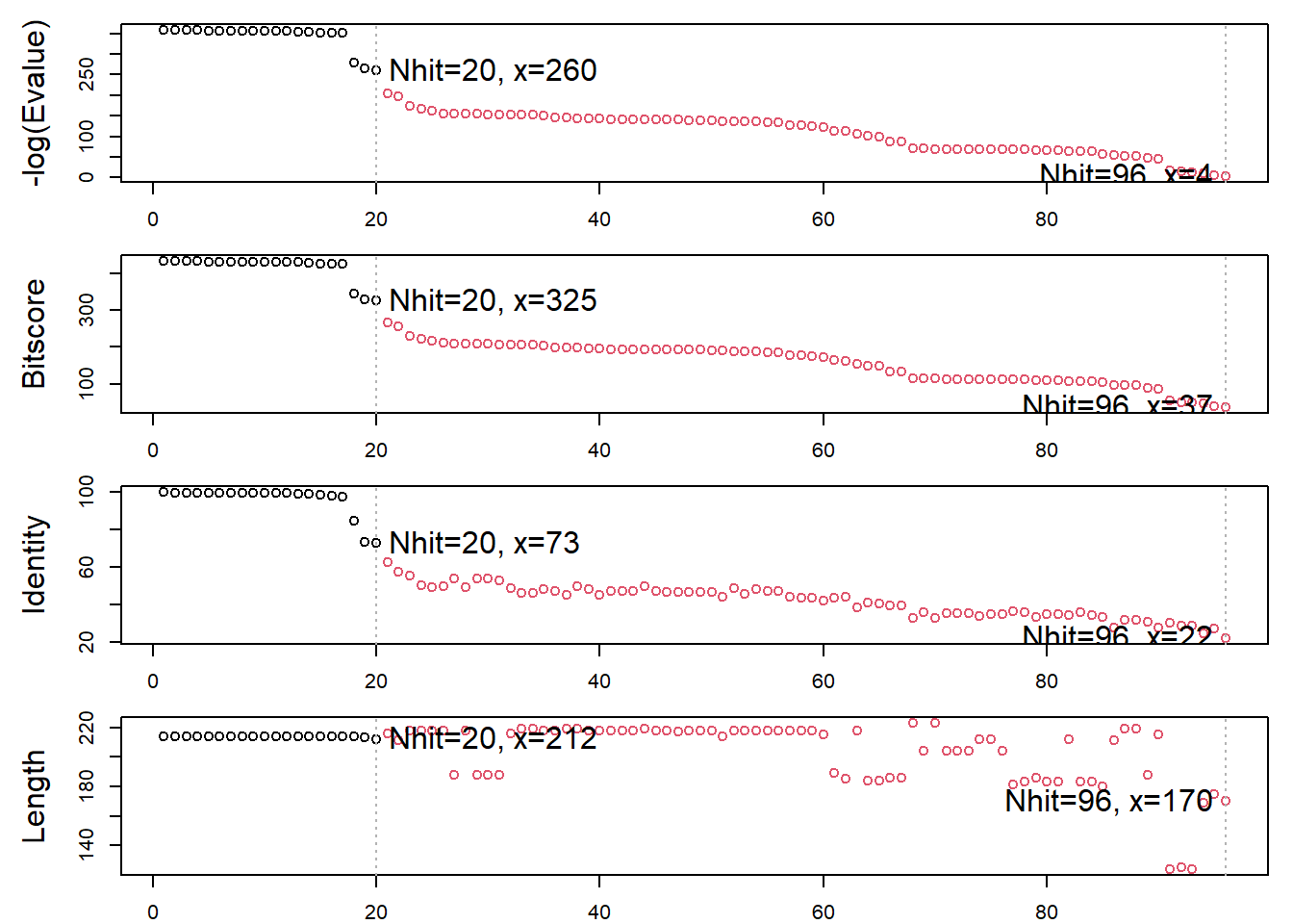
pdbs <-pdbaln(files, fit=TRUE, exefile="msa")
Reading PDB files:
pdbs/split_chain/1AKE_A.pdb
pdbs/split_chain/8BQF_A.pdb
pdbs/split_chain/4X8M_A.pdb
pdbs/split_chain/6S36_A.pdb
pdbs/split_chain/9R6U_A.pdb
pdbs/split_chain/9R71_A.pdb
pdbs/split_chain/8Q2B_A.pdb
pdbs/split_chain/8RJ9_A.pdb
pdbs/split_chain/6RZE_A.pdb
pdbs/split_chain/4X8H_A.pdb
pdbs/split_chain/3HPR_A.pdb
pdbs/split_chain/1E4V_A.pdb
pdbs/split_chain/5EJE_A.pdb
pdbs/split_chain/1E4Y_A.pdb
pdbs/split_chain/3X2S_A.pdb
pdbs/split_chain/6HAP_A.pdb
pdbs/split_chain/6HAM_A.pdb
pdbs/split_chain/8PVW_A.pdb
pdbs/split_chain/4K46_A.pdb
pdbs/split_chain/4NP6_A.pdb
   PDB has ALT records, taking A only, rm.alt=TRUE
.   PDB has ALT records, taking A only, rm.alt=TRUE
..   PDB has ALT records, taking A only, rm.alt=TRUE
.   PDB has ALT records, taking A only, rm.alt=TRUE
.   PDB has ALT records, taking A only, rm.alt=TRUE
.   PDB has ALT records, taking A only, rm.alt=TRUE
.   PDB has ALT records, taking A only, rm.alt=TRUE
.   PDB has ALT records, taking A only, rm.alt=TRUE
..   PDB has ALT records, taking A only, rm.alt=TRUE
..   PDB has ALT records, taking A only, rm.alt=TRUE
....   PDB has ALT records, taking A only, rm.alt=TRUE
.   PDB has ALT records, taking A only, rm.alt=TRUE
.   PDB has ALT records, taking A only, rm.alt=TRUE
..

Extracting sequences

pdb/seq: 1   name: pdbs/split_chain/1AKE_A.pdb
   PDB has ALT records, taking A only, rm.alt=TRUE
pdb/seq: 2   name: pdbs/split_chain/8BQF_A.pdb
   PDB has ALT records, taking A only, rm.alt=TRUE
pdb/seq: 3   name: pdbs/split_chain/4X8M_A.pdb
pdb/seq: 4   name: pdbs/split_chain/6S36_A.pdb
   PDB has ALT records, taking A only, rm.alt=TRUE
pdb/seq: 5   name: pdbs/split_chain/9R6U_A.pdb
   PDB has ALT records, taking A only, rm.alt=TRUE
pdb/seq: 6   name: pdbs/split_chain/9R71_A.pdb
   PDB has ALT records, taking A only, rm.alt=TRUE
pdb/seq: 7   name: pdbs/split_chain/8Q2B_A.pdb
   PDB has ALT records, taking A only, rm.alt=TRUE
pdb/seq: 8   name: pdbs/split_chain/8RJ9_A.pdb
   PDB has ALT records, taking A only, rm.alt=TRUE
pdb/seq: 9   name: pdbs/split_chain/6RZE_A.pdb
   PDB has ALT records, taking A only, rm.alt=TRUE
pdb/seq: 10   name: pdbs/split_chain/4X8H_A.pdb
pdb/seq: 11   name: pdbs/split_chain/3HPR_A.pdb
   PDB has ALT records, taking A only, rm.alt=TRUE
pdb/seq: 12   name: pdbs/split_chain/1E4V_A.pdb
pdb/seq: 13   name: pdbs/split_chain/5EJE_A.pdb
   PDB has ALT records, taking A only, rm.alt=TRUE
pdb/seq: 14   name: pdbs/split_chain/1E4Y_A.pdb
pdb/seq: 15   name: pdbs/split_chain/3X2S_A.pdb
pdb/seq: 16   name: pdbs/split_chain/6HAP_A.pdb
pdb/seq: 17   name: pdbs/split_chain/6HAM_A.pdb
   PDB has ALT records, taking A only, rm.alt=TRUE
pdb/seq: 18   name: pdbs/split_chain/8PVW_A.pdb
   PDB has ALT records, taking A only, rm.alt=TRUE
pdb/seq: 19   name: pdbs/split_chain/4K46_A.pdb
   PDB has ALT records, taking A only, rm.alt=TRUE
pdb/seq: 20   name: pdbs/split_chain/4NP6_A.pdb
Let’s have a peak at our structures after “fitting” or superposing:
library(bio3dview)view.pdbs(pdbs)
view.pdbs(pdbs, colorScheme="residue")
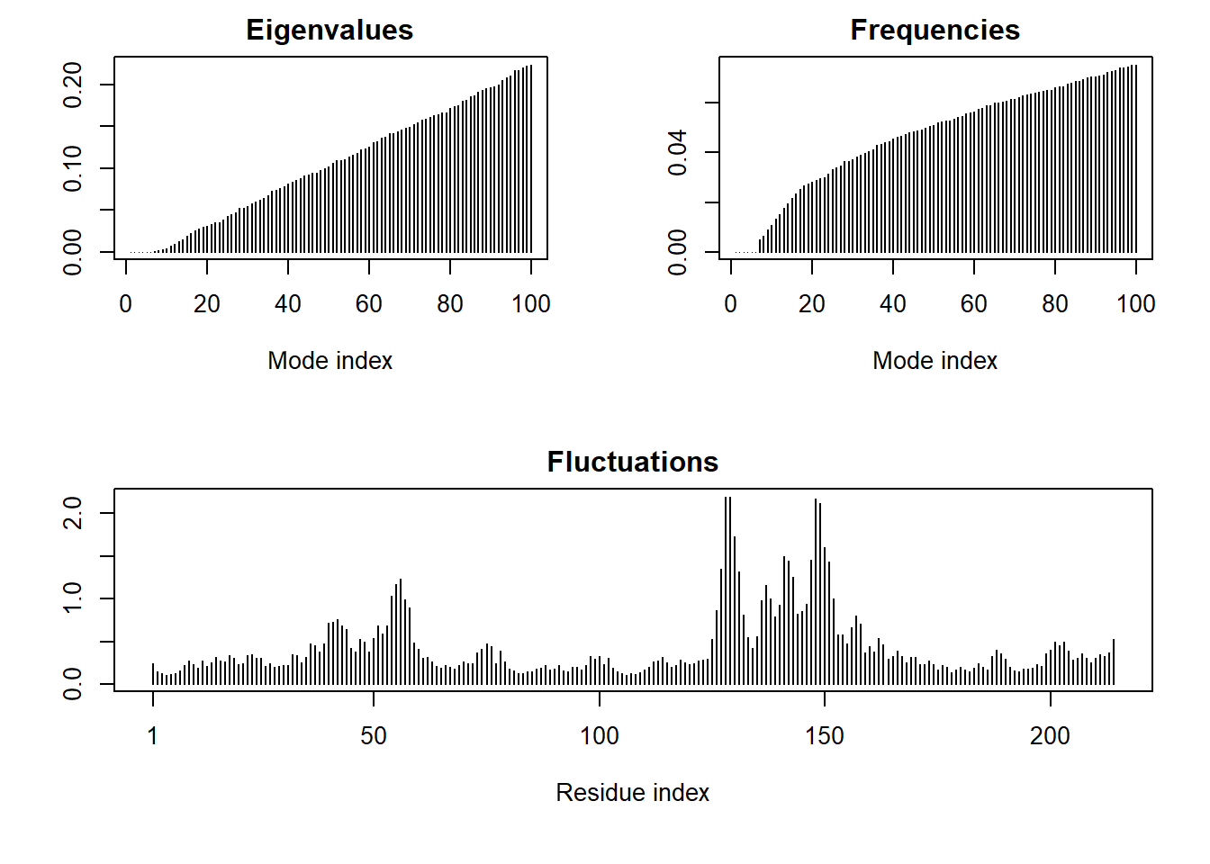
We can run functions like rmsd(), rmsf(), and the best pca()
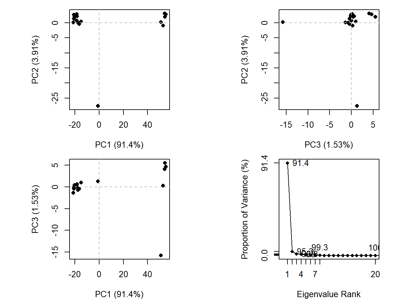
pc.xray <-pca(pdbs)plot(pc.xray)
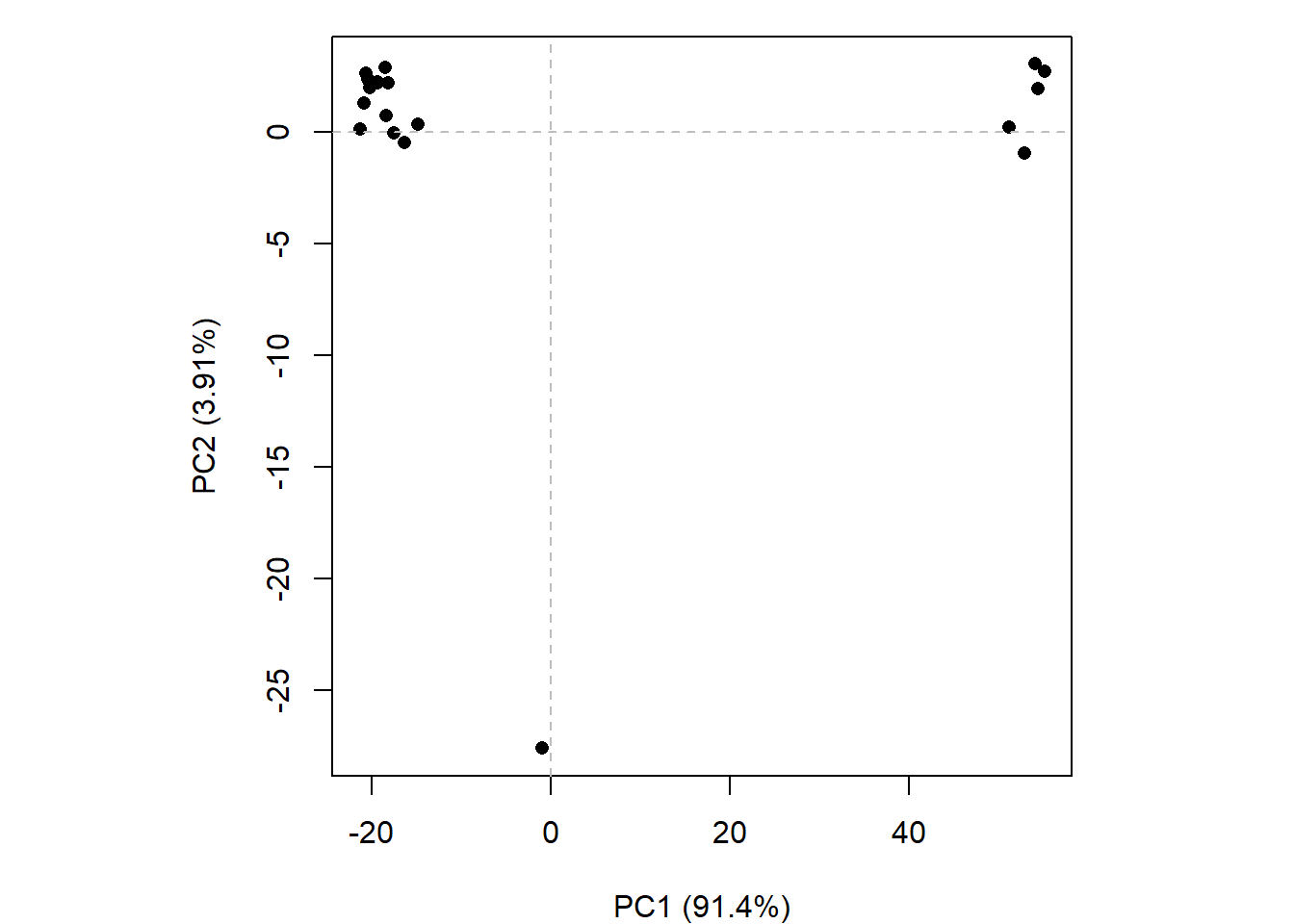
plot(pc.xray, 1:2)
Finally, let’s make a movie of the major “motion” or structural difference in the dataset - we call this a “trajectory”