countData <- read.csv("GSE37704_featurecounts.csv", row.names = 1)
metadata <- read.csv("GSE37704_metadata.csv")Class 14: RNASeq Mini-Project
Background
The data for today’s mini-project comes from a knock-down study of an important HOX gene.
Data Import
head(countData) length SRR493366 SRR493367 SRR493368 SRR493369 SRR493370
ENSG00000186092 918 0 0 0 0 0
ENSG00000279928 718 0 0 0 0 0
ENSG00000279457 1982 23 28 29 29 28
ENSG00000278566 939 0 0 0 0 0
ENSG00000273547 939 0 0 0 0 0
ENSG00000187634 3214 124 123 205 207 212
SRR493371
ENSG00000186092 0
ENSG00000279928 0
ENSG00000279457 46
ENSG00000278566 0
ENSG00000273547 0
ENSG00000187634 258metadata id condition
1 SRR493366 control_sirna
2 SRR493367 control_sirna
3 SRR493368 control_sirna
4 SRR493369 hoxa1_kd
5 SRR493370 hoxa1_kd
6 SRR493371 hoxa1_kdClean-up (data-tidying)
The metadata doesn’t match the countdata so the first column needs to be deleted for the samples names to match
Q. Complete the code below to remove the troublesome first column from
countData
countData <- countData[, -1]

head(countData)
SRR493366 SRR493367 SRR493368 SRR493369 SRR493370 SRR493371
ENSG00000186092 0 0 0 0 0 0
ENSG00000279928 0 0 0 0 0 0
ENSG00000279457 23 28 29 29 28 46
ENSG00000278566 0 0 0 0 0 0
ENSG00000273547 0 0 0 0 0 0
ENSG00000187634 124 123 205 207 212 258ncol(countData) == nrow(metadata)[1] TRUEcolnames(countData) == metadata$id[1] TRUE TRUE TRUE TRUE TRUE TRUENow we have to remove rows where all the samples have a value of 0 because they contain no data
Q. Complete the code below to filter countData to exclude genes (i.e. rows) where we have 0 read count across all samples (i.e. columns).
countData = countData[rowSums(countData) > 0, ]
head(countData)
SRR493366 SRR493367 SRR493368 SRR493369 SRR493370 SRR493371
ENSG00000279457 23 28 29 29 28 46
ENSG00000187634 124 123 205 207 212 258
ENSG00000188976 1637 1831 2383 1226 1326 1504
ENSG00000187961 120 153 180 236 255 357
ENSG00000187583 24 48 65 44 48 64
ENSG00000187642 4 9 16 14 16 16DESeq Analysis
library(DESeq2)Setting up the DESeq object
dds <- DESeqDataSetFromMatrix(countData= countData,
                       colData =  metadata,
                       design = ~condition)
Warning in DESeqDataSet(se, design = design, ignoreRank): some variables in
design formula are characters, converting to factorsRunning DESeq
dds <- DESeq(dds)estimating size factorsestimating dispersionsgene-wise dispersion estimatesmean-dispersion relationshipfinal dispersion estimatesfitting model and testingres <- results(dds)
head(res)log2 fold change (MLE): condition hoxa1 kd vs control sirna
Wald test p-value: condition hoxa1 kd vs control sirna
DataFrame with 6 rows and 6 columns
baseMean log2FoldChange lfcSE stat pvalue
<numeric> <numeric> <numeric> <numeric> <numeric>
ENSG00000279457 29.9136 0.1792571 0.3248216 0.551863 5.81042e-01
ENSG00000187634 183.2296 0.4264571 0.1402658 3.040350 2.36304e-03
ENSG00000188976 1651.1881 -0.6927205 0.0548465 -12.630158 1.43990e-36
ENSG00000187961 209.6379 0.7297556 0.1318599 5.534326 3.12428e-08
ENSG00000187583 47.2551 0.0405765 0.2718928 0.149237 8.81366e-01
ENSG00000187642 11.9798 0.5428105 0.5215598 1.040744 2.97994e-01
padj
<numeric>
ENSG00000279457 6.86555e-01
ENSG00000187634 5.15718e-03
ENSG00000188976 1.76549e-35
ENSG00000187961 1.13413e-07
ENSG00000187583 9.19031e-01
ENSG00000187642 4.03379e-01Getting results
Q. Call the summary() function on your results to get a sense of how many genes are up or down-regulated at the default 0.1 p-value cutoff.
summary(res)
out of 15975 with nonzero total read count
adjusted p-value < 0.1
LFC > 0 (up)       : 4349, 27%
LFC < 0 (down)     : 4396, 28%
outliers [1]       : 0, 0%
low counts [2]     : 1237, 7.7%
(mean count < 0)
[1] see 'cooksCutoff' argument of ?results
[2] see 'independentFiltering' argument of ?results
Volcano Plot
A plot of log2 fold change vs -log of Adjusted P-value
library(ggplot2)ggplot(res) +
aes(log2FoldChange, -log(padj)) +
geom_point() +
geom_hline(yintercept=-log(0.01), col="red")Warning: Removed 1237 rows containing missing values or values outside the scale range
(`geom_point()`).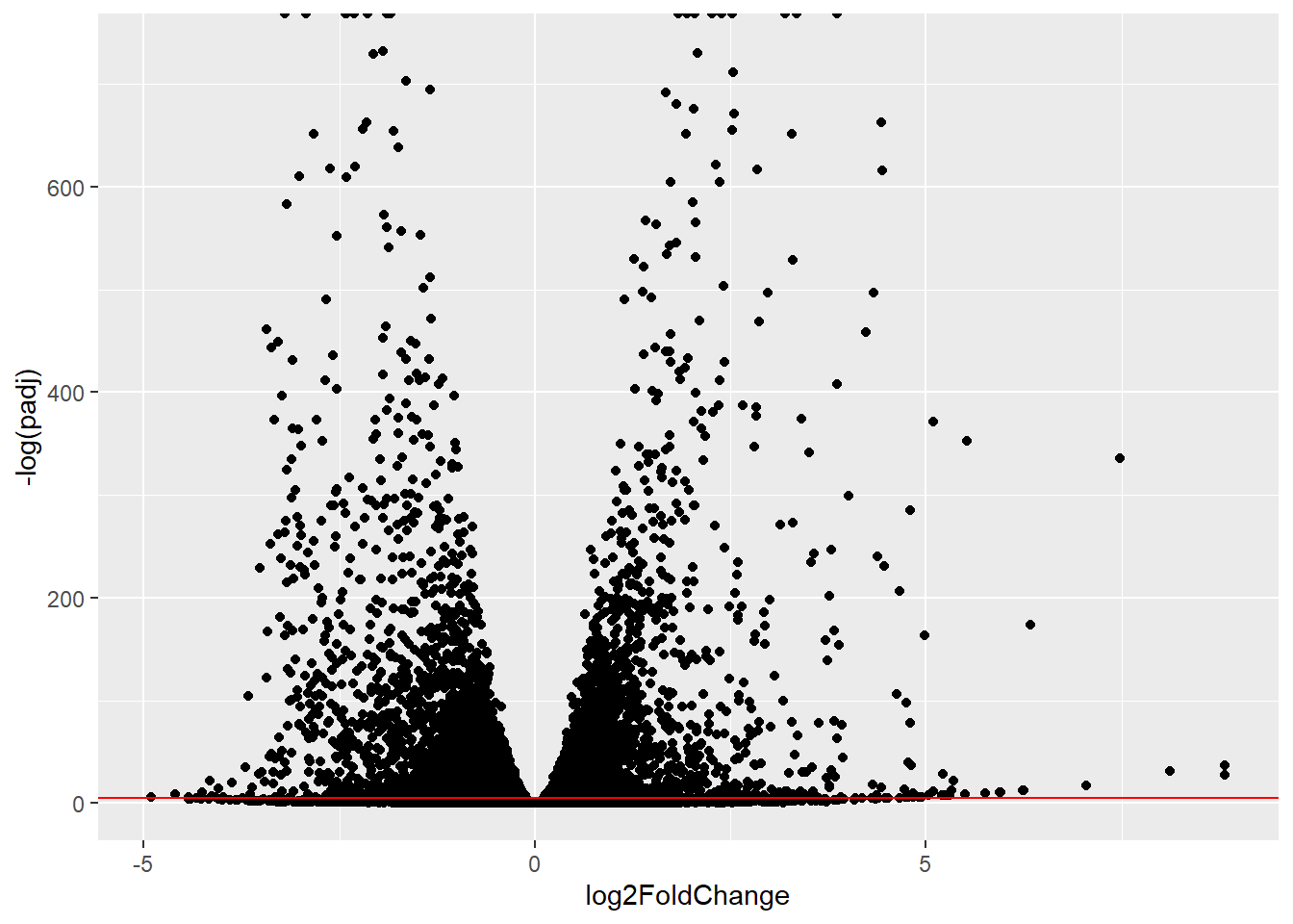
Q. Improve this plot by completing the below code, which adds color, axis labels and cutoff lines:
mycols <- rep("grey", nrow(res))
mycols[abs(res$log2FoldChange) >2] <- "darkblue"
mycols[res$padj >= 0.01] <- "gray"

ggplot(res) +
  aes(log2FoldChange, -log(padj)) +
  geom_point(col=mycols) +
  geom_vline(xintercept = c(-2,+2), col="red") +
  geom_hline(yintercept=-log(0.01), col="red") +
    ylab("log(Adjusted P-value") + xlab("Fold change") +
  labs(title="Effects of Expression of HOX")
Warning: Removed 1237 rows containing missing values or values outside the scale range
(`geom_point()`).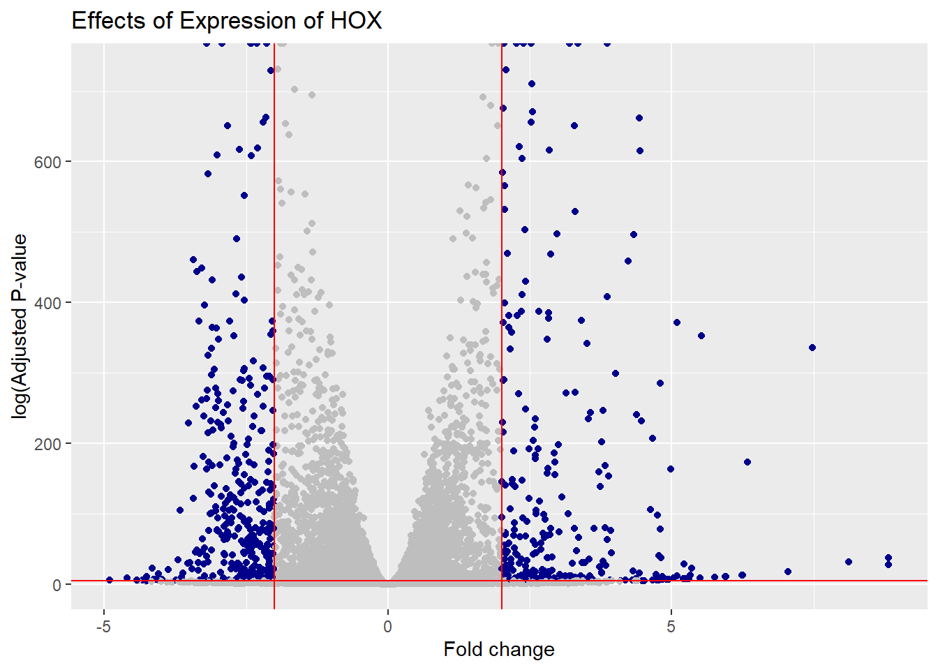
Add Annotation
Q. Use the mapIDs() function multiple times to add SYMBOL, ENTREZID and GENENAME annotation to our results by completing the code below.
library("AnnotationDbi")
library("org.Hs.eg.db")columns(org.Hs.eg.db) [1] "ACCNUM" "ALIAS" "ENSEMBL" "ENSEMBLPROT" "ENSEMBLTRANS"
[6] "ENTREZID" "ENZYME" "EVIDENCE" "EVIDENCEALL" "GENENAME"
[11] "GENETYPE" "GO" "GOALL" "IPI" "MAP"
[16] "OMIM" "ONTOLOGY" "ONTOLOGYALL" "PATH" "PFAM"
[21] "PMID" "PROSITE" "REFSEQ" "SYMBOL" "UCSCKG"
[26] "UNIPROT" res$symbol = mapIds(org.Hs.eg.db,
keys=rownames(res),
keytype="ENSEMBL",
column="SYMBOL")'select()' returned 1:many mapping between keys and columnsres$entrez = mapIds(org.Hs.eg.db,
keys=rownames(res),
keytype="ENSEMBL",
column="ENTREZID",)'select()' returned 1:many mapping between keys and columnsres$name = mapIds(org.Hs.eg.db,
keys=row.names(res),
keytype="ENSEMBL",
column="GENENAME")'select()' returned 1:many mapping between keys and columnshead(res)log2 fold change (MLE): condition hoxa1 kd vs control sirna
Wald test p-value: condition hoxa1 kd vs control sirna
DataFrame with 6 rows and 9 columns
baseMean log2FoldChange lfcSE stat pvalue
<numeric> <numeric> <numeric> <numeric> <numeric>
ENSG00000279457 29.9136 0.1792571 0.3248216 0.551863 5.81042e-01
ENSG00000187634 183.2296 0.4264571 0.1402658 3.040350 2.36304e-03
ENSG00000188976 1651.1881 -0.6927205 0.0548465 -12.630158 1.43990e-36
ENSG00000187961 209.6379 0.7297556 0.1318599 5.534326 3.12428e-08
ENSG00000187583 47.2551 0.0405765 0.2718928 0.149237 8.81366e-01
ENSG00000187642 11.9798 0.5428105 0.5215598 1.040744 2.97994e-01
padj symbol entrez name
<numeric> <character> <character> <character>
ENSG00000279457 6.86555e-01 NA NA NA
ENSG00000187634 5.15718e-03 SAMD11 148398 sterile alpha motif ..
ENSG00000188976 1.76549e-35 NOC2L 26155 NOC2 like nucleolar ..
ENSG00000187961 1.13413e-07 KLHL17 339451 kelch like family me..
ENSG00000187583 9.19031e-01 PLEKHN1 84069 pleckstrin homology ..
ENSG00000187642 4.03379e-01 PERM1 84808 PPARGC1 and ESRR ind..Q. Finally for this section let’s reorder these results by adjusted p-value and save them to a CSV file in your current project directory.
res = res[order(res$pvalue),]
write.csv(res, file = "deseq_results.csv")
Pathway Analysis
library(pathview)
library(gage)
library(gageData)

data(kegg.sets.hs)
data(sigmet.idx.hs)

kegg.sets.hs = kegg.sets.hs[sigmet.idx.hs]
We need a foldchanges vector for gage()
foldchanges <- res$log2FoldChange
names(foldchanges) <- res$entrez
head(foldchanges)
1266 54855 1465 2034 2150 6659
-2.422719 3.201955 -2.313738 -1.888019 3.344508 2.392288 keggres = gage(foldchanges, gsets=kegg.sets.hs)KEGG
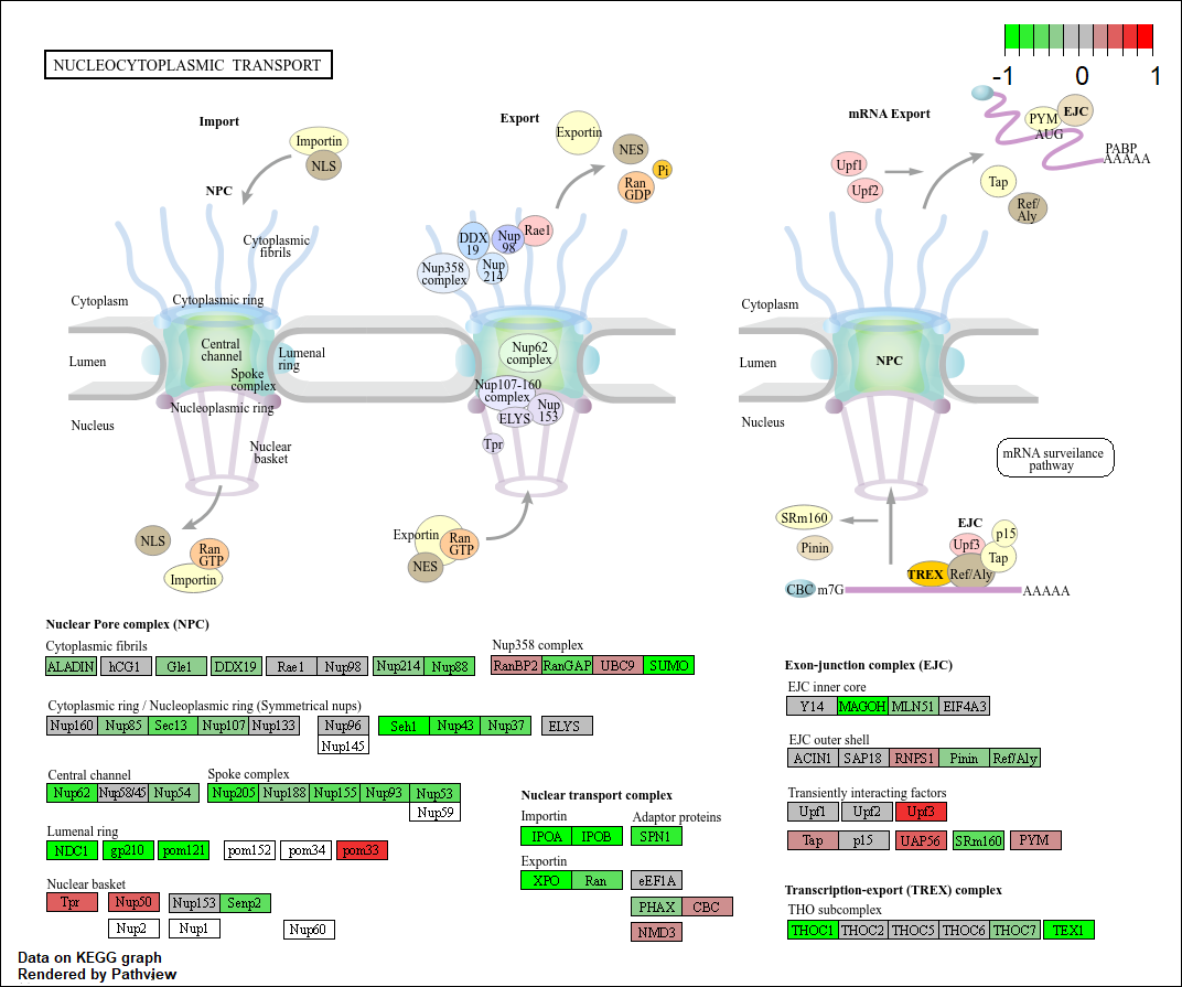
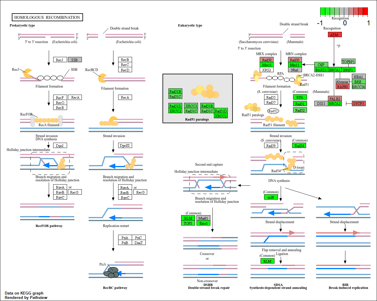
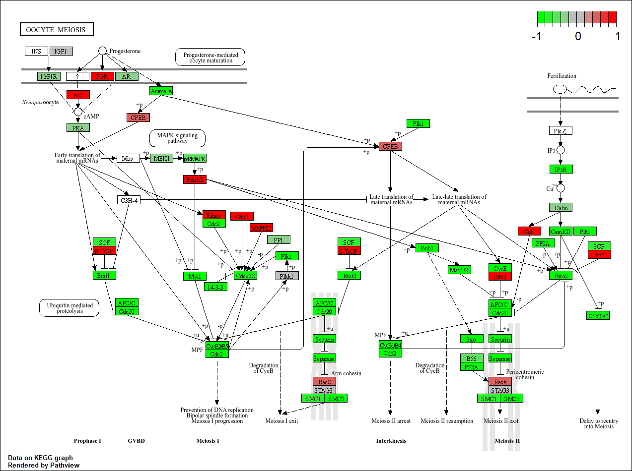
Q. Can you plot the pathview figures for the top 5 down-regulated pathways?
head(keggres$less, 5) p.geomean stat.mean p.val
hsa04110 Cell cycle 8.995727e-06 -4.378644 8.995727e-06
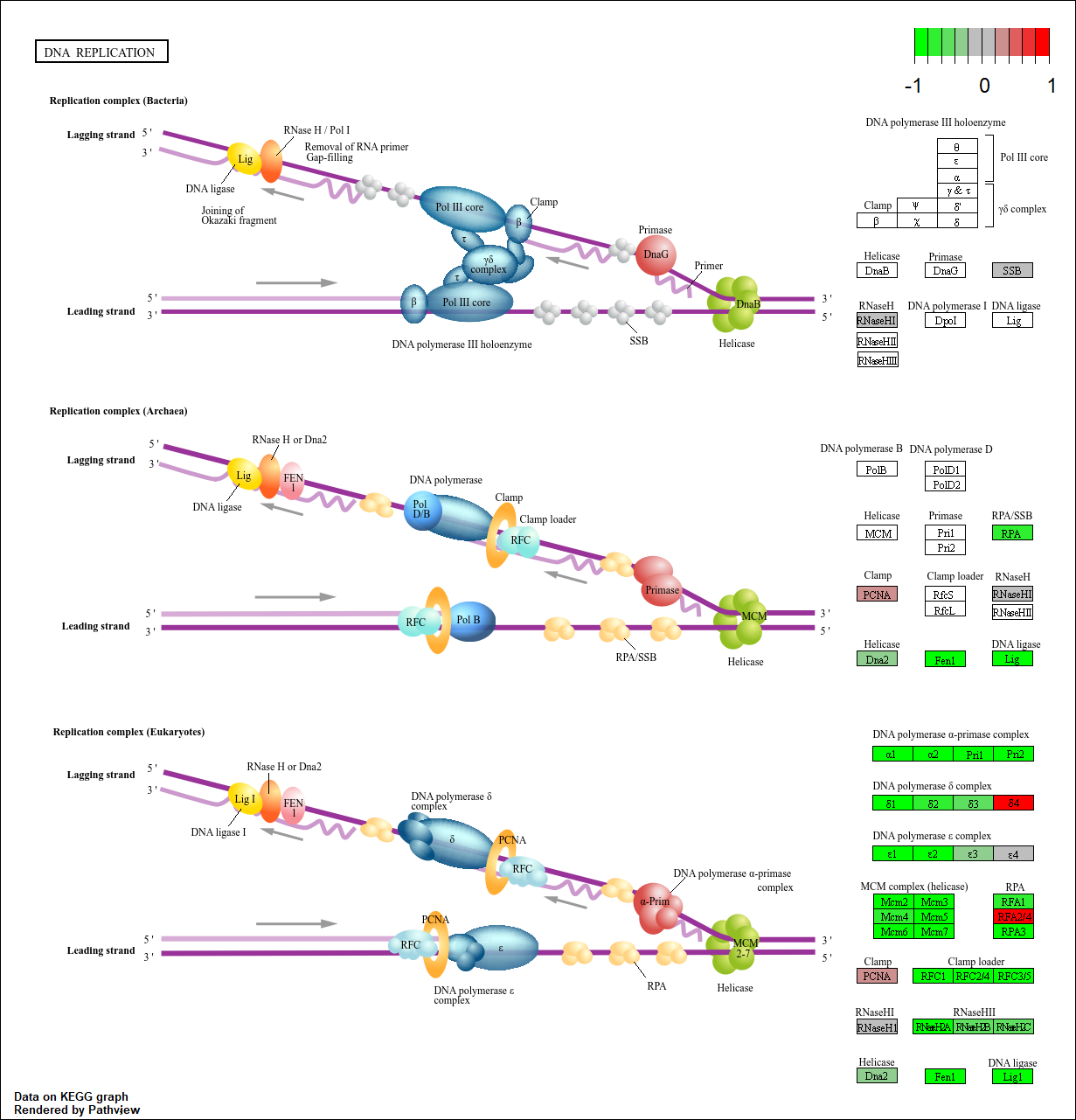
hsa03030 DNA replication 9.424076e-05 -3.951803 9.424076e-05
hsa03013 RNA transport 1.375901e-03 -3.028500 1.375901e-03
hsa03440 Homologous recombination 3.066756e-03 -2.852899 3.066756e-03
hsa04114 Oocyte meiosis 3.784520e-03 -2.698128 3.784520e-03
q.val set.size exp1
hsa04110 Cell cycle 0.001448312 121 8.995727e-06
hsa03030 DNA replication 0.007586381 36 9.424076e-05
hsa03013 RNA transport 0.073840037 144 1.375901e-03
hsa03440 Homologous recombination 0.121861535 28 3.066756e-03
hsa04114 Oocyte meiosis 0.121861535 102 3.784520e-03pathview(foldchanges, pathway.id=c("hsa04110"))
pathview(foldchanges, pathway.id=c("hsa03030"))
pathview(foldchanges, pathway.id=c("hsa03013"))
pathview(foldchanges, pathway.id=c("hsa03440"))
pathview(foldchanges, pathway.id=c("hsa04114"))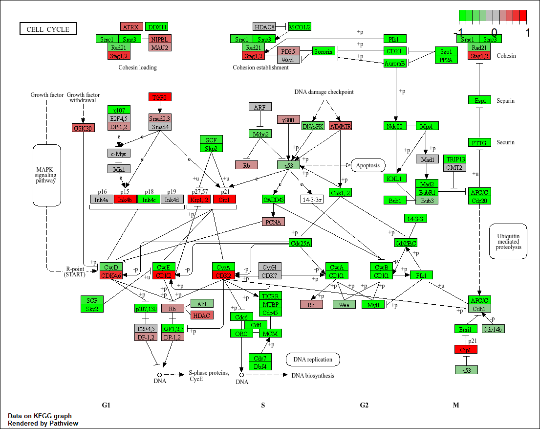
GO
data(go.sets.hs)
data(go.subs.hs)

# Biological Process subset of GO
gobpsets = go.sets.hs[go.subs.hs$BP]

gobpres = gage(foldchanges, gsets=gobpsets)

lapply(gobpres, head)
$greater
p.geomean stat.mean p.val
GO:0007156 homophilic cell adhesion 8.519724e-05 3.824205 8.519724e-05
GO:0002009 morphogenesis of an epithelium 1.396681e-04 3.653886 1.396681e-04
GO:0048729 tissue morphogenesis 1.432451e-04 3.643242 1.432451e-04
GO:0007610 behavior 1.925222e-04 3.565432 1.925222e-04
GO:0060562 epithelial tube morphogenesis 5.932837e-04 3.261376 5.932837e-04
GO:0035295 tube development 5.953254e-04 3.253665 5.953254e-04
q.val set.size exp1
GO:0007156 homophilic cell adhesion 0.1951953 113 8.519724e-05
GO:0002009 morphogenesis of an epithelium 0.1951953 339 1.396681e-04
GO:0048729 tissue morphogenesis 0.1951953 424 1.432451e-04
GO:0007610 behavior 0.1967577 426 1.925222e-04
GO:0060562 epithelial tube morphogenesis 0.3565320 257 5.932837e-04
GO:0035295 tube development 0.3565320 391 5.953254e-04
$less
p.geomean stat.mean p.val
GO:0048285 organelle fission 1.536227e-15 -8.063910 1.536227e-15
GO:0000280 nuclear division 4.286961e-15 -7.939217 4.286961e-15
GO:0007067 mitosis 4.286961e-15 -7.939217 4.286961e-15
GO:0000087 M phase of mitotic cell cycle 1.169934e-14 -7.797496 1.169934e-14
GO:0007059 chromosome segregation 2.028624e-11 -6.878340 2.028624e-11
GO:0000236 mitotic prometaphase 1.729553e-10 -6.695966 1.729553e-10
q.val set.size exp1
GO:0048285 organelle fission 5.841698e-12 376 1.536227e-15
GO:0000280 nuclear division 5.841698e-12 352 4.286961e-15
GO:0007067 mitosis 5.841698e-12 352 4.286961e-15
GO:0000087 M phase of mitotic cell cycle 1.195672e-11 362 1.169934e-14
GO:0007059 chromosome segregation 1.658603e-08 142 2.028624e-11
GO:0000236 mitotic prometaphase 1.178402e-07 84 1.729553e-10
$stats
stat.mean exp1
GO:0007156 homophilic cell adhesion 3.824205 3.824205
GO:0002009 morphogenesis of an epithelium 3.653886 3.653886
GO:0048729 tissue morphogenesis 3.643242 3.643242
GO:0007610 behavior 3.565432 3.565432
GO:0060562 epithelial tube morphogenesis 3.261376 3.261376
GO:0035295 tube development 3.253665 3.253665Reactome
sig_genes <- res[res$padj <= 0.05 & !is.na(res$padj), "symbol"]
print(paste("Total number of significant genes:", length(sig_genes)))
[1] "Total number of significant genes: 8147"write.table(sig_genes, file="significant_genes.txt", row.names=FALSE, col.names=FALSE, quote=FALSE)Q. What pathway has the most significant “Entities p-value”? Do the most significant pathways listed match your previous KEGG results? What factors could cause differences between the two methods?
Cell Cycle, Mitotic had the most significant entities p-value, and this matches with the previous KEGG results to the extent that they are both cell cycle. Reactome lists cell cycle as the second most significant. Factors that could cause differences it is how specific into each pathway KEGG and Reactome get, in which are they considering the pathway as a whole or breaking the pathway into separate parts.