Class 17: Analyzing Sequencing Data in Cloud

Downstream Analysis

library(tximport)

folders <- dir(pattern="SRR21568*")
samples <- sub("_quant", "", folders)
files <- file.path(folders, "abundance.h5")
names(files) <- samples
txi.kallisto <- tximport(files, type = "kallisto", txOut = TRUE)

1 2 3 4 

head(txi.kallisto$counts)

                SRR2156848 SRR2156849 SRR2156850 SRR2156851
ENST00000539570          0          0    0.00000          0
ENST00000576455          0          0    2.62037          0
ENST00000510508          0          0    0.00000          0
ENST00000474471          0          1    1.00000          0
ENST00000381700          0          0    0.00000          0
ENST00000445946          0          0    0.00000          0

colSums(txi.kallisto$counts)

SRR2156848 SRR2156849 SRR2156850 SRR2156851 
   2563611    2600800    2372309    2111474 

sum(rowSums(txi.kallisto$counts)>0)

[1] 94561

to.keep <- rowSums(txi.kallisto$counts) > 0
kset.nonzero <- txi.kallisto$counts[to.keep,]
keep2 <- apply(kset.nonzero,1,sd)>0
x <- kset.nonzero[keep2,]

PCA

pca <- prcomp(t(x), scale=TRUE)
summary(pca)

Importance of components:
                            PC1      PC2      PC3   PC4
Standard deviation     183.6379 177.3605 171.3020 1e+00
Proportion of Variance   0.3568   0.3328   0.3104 1e-05
Cumulative Proportion    0.3568   0.6895   1.0000 1e+00

plot(pca$x[,1], pca$x[,2],
     col=c("blue","blue","red","red"),
     xlab="PC1", ylab="PC2", pch=16)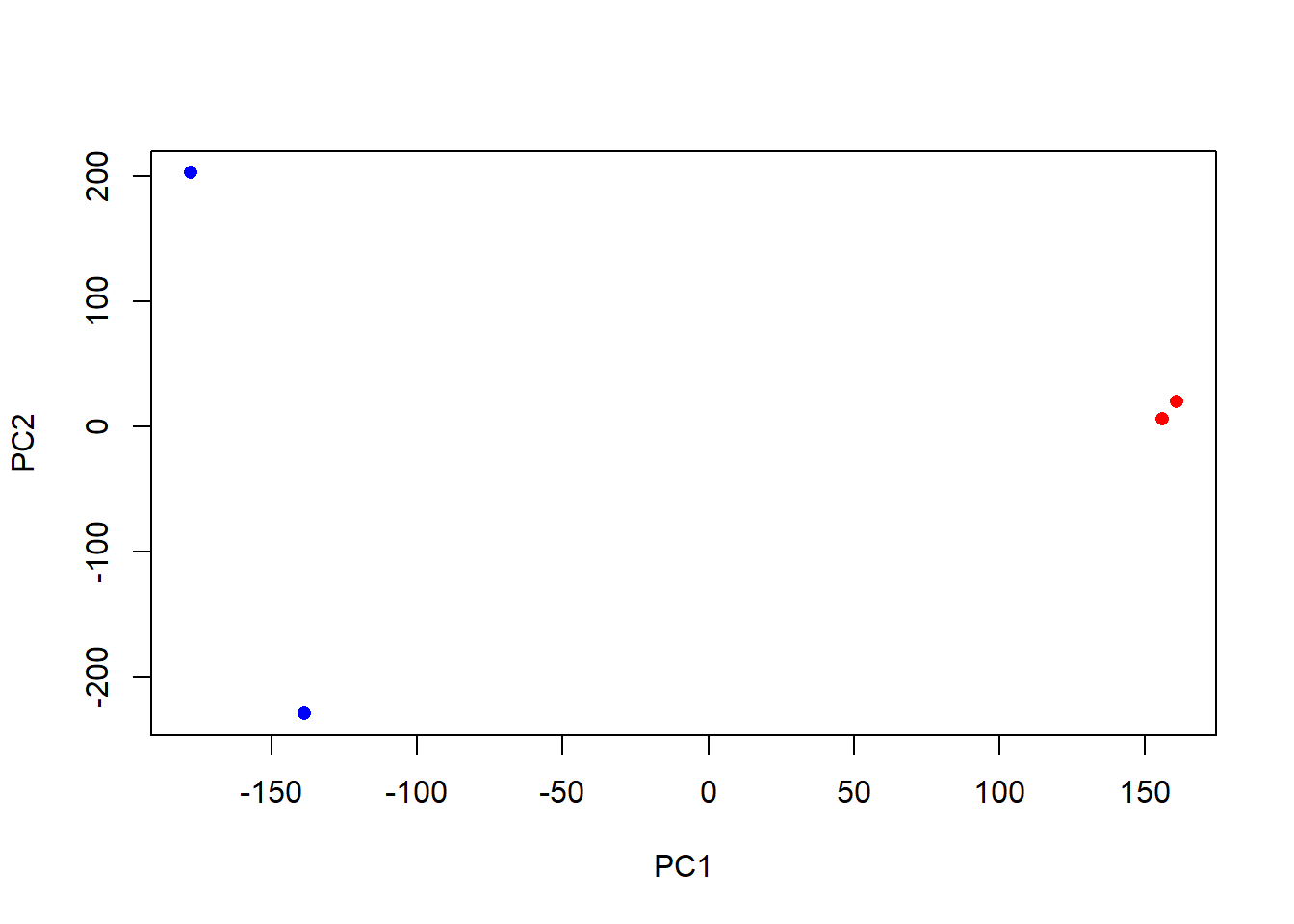

library(ggplot2)

Q. Use ggplot to make a similar figure of PC1 and PC2

ggplot(pca$x) +
  aes(PC1, PC2) +
  geom_point(col=c("blue","blue","red","red"))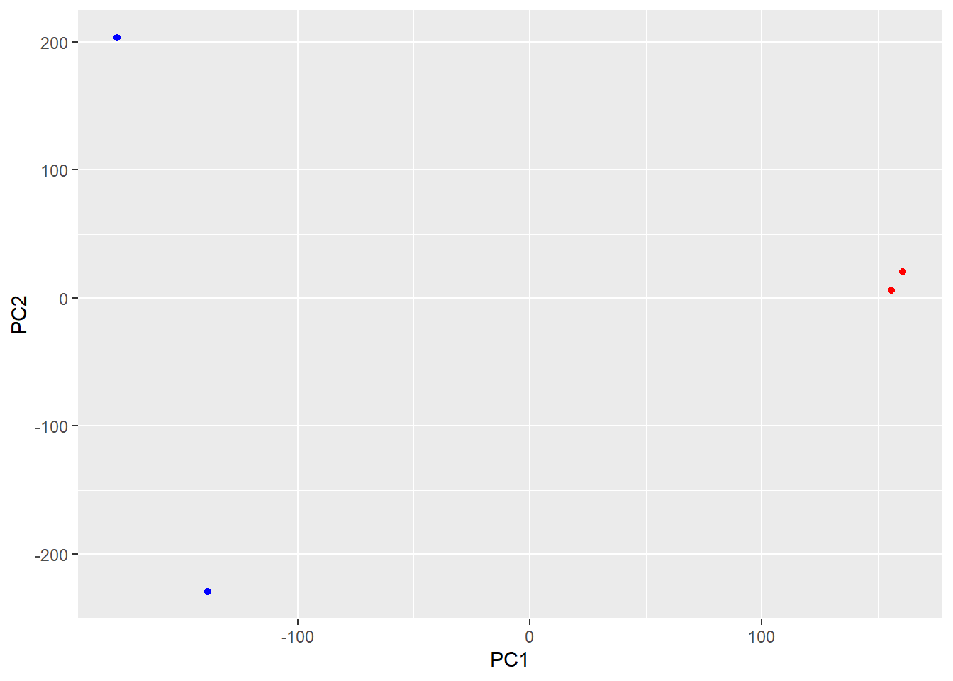

Q. a separate figure PC1 vs PC3

ggplot(pca$x) +
  aes(PC1, PC3) +
  geom_point(col=c("blue","blue","red","red"))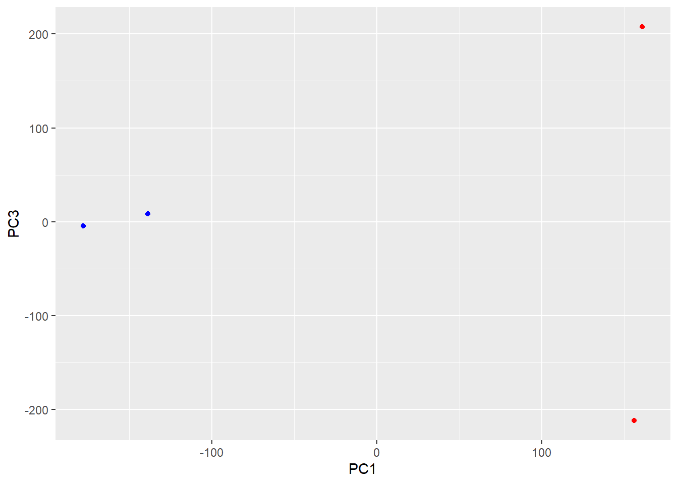

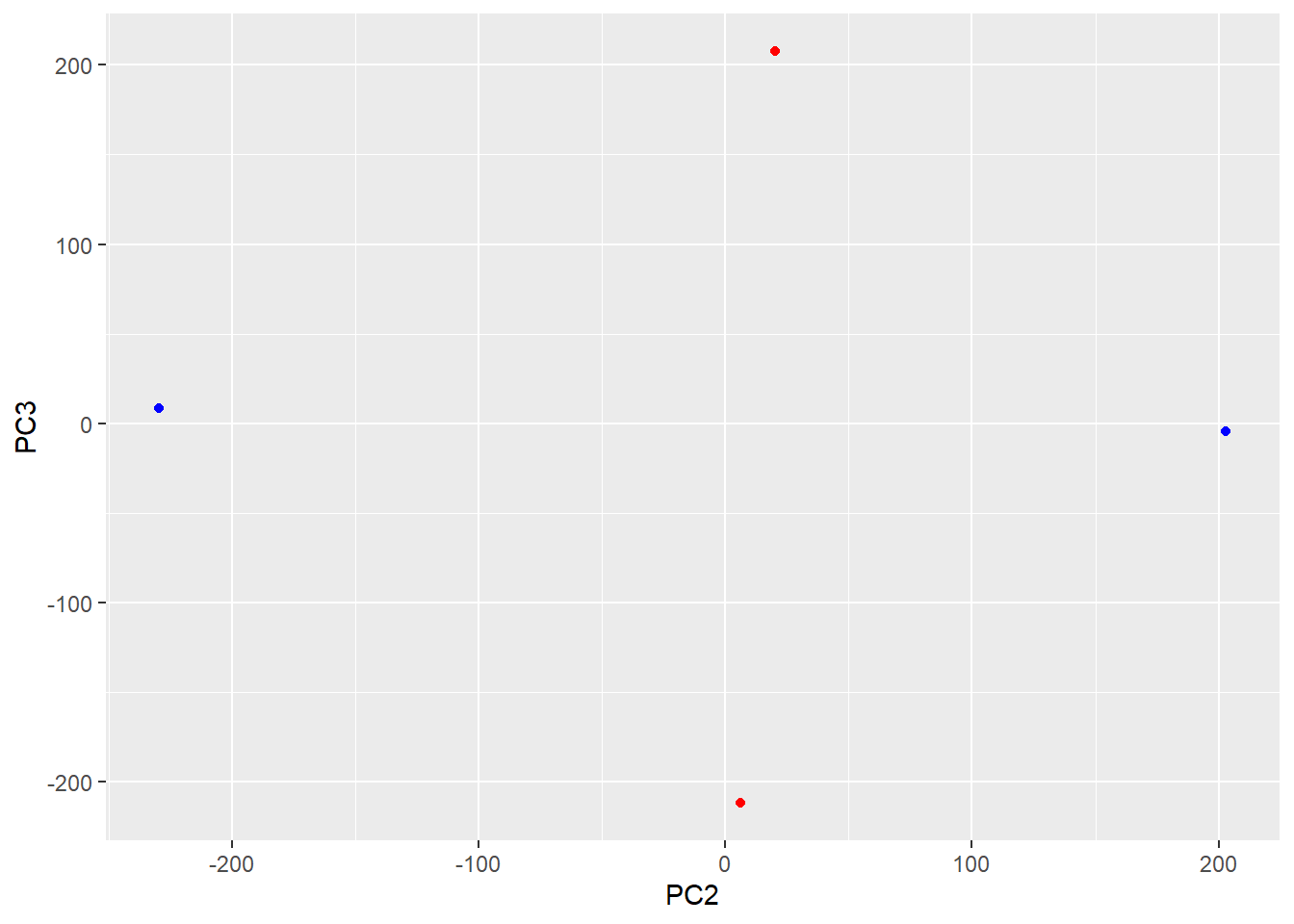
Q. and PC2 vs PC3

ggplot(pca$x) +
  aes(PC2, PC3) +
  geom_point(col=c("blue","blue","red","red"))